In the previous blog, we gained an understanding on how Artificial Neural Network (ANN) iterates in a loop of forward & backward propagation in order to minimize the error between the predicted output & the actual output. This article will cover Gradient descent, an optimization algorithm that is used when training an Artificial Neural Network (ANN). Before understanding how Gradient Descent works, let’s explore the idea behind what is optimization and how optimizers actually work?

Working of Optimizers

The process of minimizing any mathematical expression is referred to as Optimization. Optimizers are algorithms employed to change the parameters of the neural network such as weights and bias to reduce the losses.

• ANN starts with the initial random guess of weights and biases and calculates the output (predicted output) in a feedforward propagation. It is impossible to know the exact best estimates of weights and biases from the start itself, such that the predicted output matches with the actual output.

• ANN then back propagates the resulting gradient of the loss with respect to weights and biases across each layer of ANN (backward) to minimize the loss function.

• The process of reducing the loss is defined by the optimizers. The optimizers change the parameters of ANN iteratively over the training cycles in order to obtain the minimum loss.

• There are several optimizers that are being used in ANN. Few examples of commonly used optimizers are Gradient Descent (GD), Stochastic Gradient Descent (SGD), Mini-batch Gradient Descent (MB-SGD), SGD with momentum, RMSProp, and Adam, etc.

In this article, we’re going to explore the working behind the GD optimizer along with its variants - SGD and MB-SGD.

Terminologies Used in Gradient Descent (G.D) Algorithm

Loss Function: Loss function is a method of evaluating how well your algorithm models your dataset. It is a function that returns the cost associated with the model. If the value of the loss function is higher, it indicates that the model prediction is not satisfactory. The loss function is always computed for a single training example.

Cost Function: Cost function is defined as an average loss over the entire training dataset. The Cost function can be modelled in the form of mean square error as:

where, m = number of training examples     h(θ) = hypothesis (prediction) of output     y = actual output

Gradient: It refers to an inclined part of a pathway or a slope. For our ANN, we have two parameters - weights and biases, which are to be optimized to minimize the loss. So, we calculate the derivatives of a cost function with respect to both weight and bias.

Descent: To optimize the parameters of ANN, we need to descend to the point of minimum. The iterative process involved in reaching the point of minimum is called Descent.

For the sake of simplicity, we are only going to consider weight as a parameter of ANN, in understanding GD. Bias is not considered for the scope of this article.

Gradient Descent Algorithm

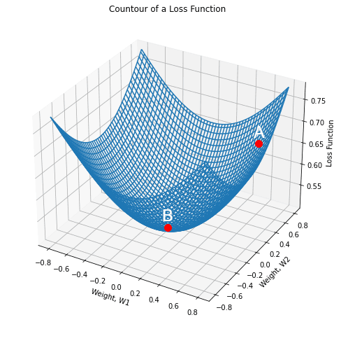
Fig1. assumes only two weight parameters: W1 and W2 for the sake of simplicity. However, ANN can have a larger number of parameters in real-time data. Here, the x-axis and the y-axis represent the values of two weights, and the z-axis represents the value of a loss function for a particular value of two weights. The goal of the Gradient Descent algorithm is to find the optimal value of weights for which the loss is minimum.

Imagine two points, A and B on the contour of fig1. Point ‘B’ is an indicative measure of the point of minimum. We want to navigate from point ‘A’ to point ‘B’, where the loss function is minimum. Two things are critical while navigating towards the global minima - the direction and the step size.

Direction: We start our search by looking at each possible direction in the x-y plane. We should consider the direction that brings about the steepest decline in the value of our loss function. We define a plane that is tangential to the point ‘A.’ We can precisely obtain one direction that will give us the direction in which the function has the steepest ascent. This direction is given by the gradient. The direction opposite to it is the direction of steepest descent. We perform descent along the direction of the gradient and the algorithm is known as Gradient Descent.

Step-size: Once we know the direction of descent, the next step is to choose the size of the steps in order to reach point ‘B.’ This is referred to as the learning rate in Gradient Descent. If we choose a very high learning rate, we may overshoot the minima and keep bouncing along the ridges of the valley and we may never reach our minima. On the other hand, if we proceed with a very small learning rate, we may increase the computational time of training.

GD Equation: The GD equation can be generalized as following: Repeat until convergence { } where the gradient of the cost function J(w)is calculated with respect to weights ‘w’ for the entire training dataset. Here, 𝝰 represents the learning rate/step size of GD.

GD - Intuition

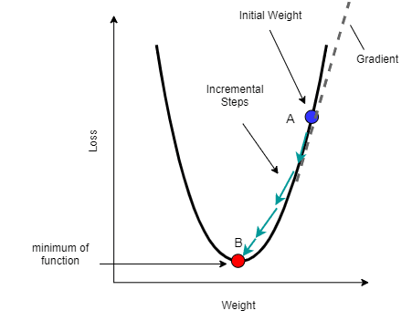
In order to understand the working logic behind GD, consider the following fig2 as a 2-D view of a representation of loss w.r.t weight. The goal of GD is to start from a point, let’s say A, and to reach the global minima as indicated by point B.

It is apparent from the fig2 that tangent to point A has a positive slope as it is a rising curve. So, if we apply our GD equation to this case then the overall value of weight or input feature will decrease, and we would move in a downward direction in the steps to reach the point of minimum.

Consider the second case as having the point ‘A’ (not shown in the figure) in the area of the upper left part, in an exactly opposite direction to point ‘A’ as shown in fig2. In that case, point A would have a negative slope and thus the gradient of cost function will be negative. But, the overall value of the slope would be positive (negative signs would cancel each other in an equation), indicating that the weight has to be increased downwards, thus pushing towards the point of minimum in the steps.

Disadvantages of GD Algorithm

1. It is computationally slower if the size of the training set is considerably large. The GD processes the entire training set before it takes a small step. Hence, GD is not efficient for processing the large dataset.

2. GD also requires a large memory to calculate the gradients of the whole dataset.

3. GD may trap at local minima and may never reach global minima. A local minimum of a function is a point where the value of the function is smaller than the value at nearby points but possibly greater than a value at some distant point. A global minimum is a point where the function value is smaller than at all other feasible points on a curve.

Variants of GD

Stochastic Gradient Descent (SGD)

SGD is an extended version of GD and it aims to overcome the disadvantages of GD. Instead of waiting to sum up the gradients over all training examples, SGD computes the gradient by taking one point at a time.

SGD takes a little step with respect to the cost of just this first training example. Then, it will modify the parameters to just fit the first training example a little bit better. SGD then would go for the second training example and take another step in the parameter space. This way, SGD continues to cover the entire training set. SGD is relatively faster than the GD algorithm.

However, SGD never converges to a minimum, it always oscillates and wanders around the region of the minimum. SGD also takes a longer time to converge in the proximity of the area of convergence.

Mini Batch Gradient Descent (MB-GD)

MB-GD is an extension of GD and it addresses the problem of large time complexity in the case of SGD. MB-GD divides the dataset into various batches and after processing each batch, the parameters are updated. The update of weight is dependent on the gradient of loss for each batch taken into consideration. Consequently, the updates in the case of MB-GD are much noisy as the gradients may not always be directed towards the minima. Moreover, it introduces one additional hyperparameter called ‘mini batch size’ that needs to be tuned properly with other parameters for achieving better performance.

Conclusion

This article covered the idea behind the working of Gradient Descent Optimizer. It also highlighted the variants of the GD algorithm in brief. Optimization is an essential process related to backpropagation in an Artificial Neural Network. The end goal of any optimizer, in general, is to minimize the cost function iteratively over time.

Gradient Descent is most suitable for the smaller training set as it could become computationally slower. SGD could be useful for larger datasets, as it can converge faster, provided it causes updates to the parameters more frequently. MB-SGD is a very popular choice for the training of deep neural networks as it is a good balance between both GD and SGD in terms of efficiency.

References:

1. Neural networks

2. Optimizers for training neural network

3. Gradient descent

4. Cost function